Architecture Details: The Two-Context System
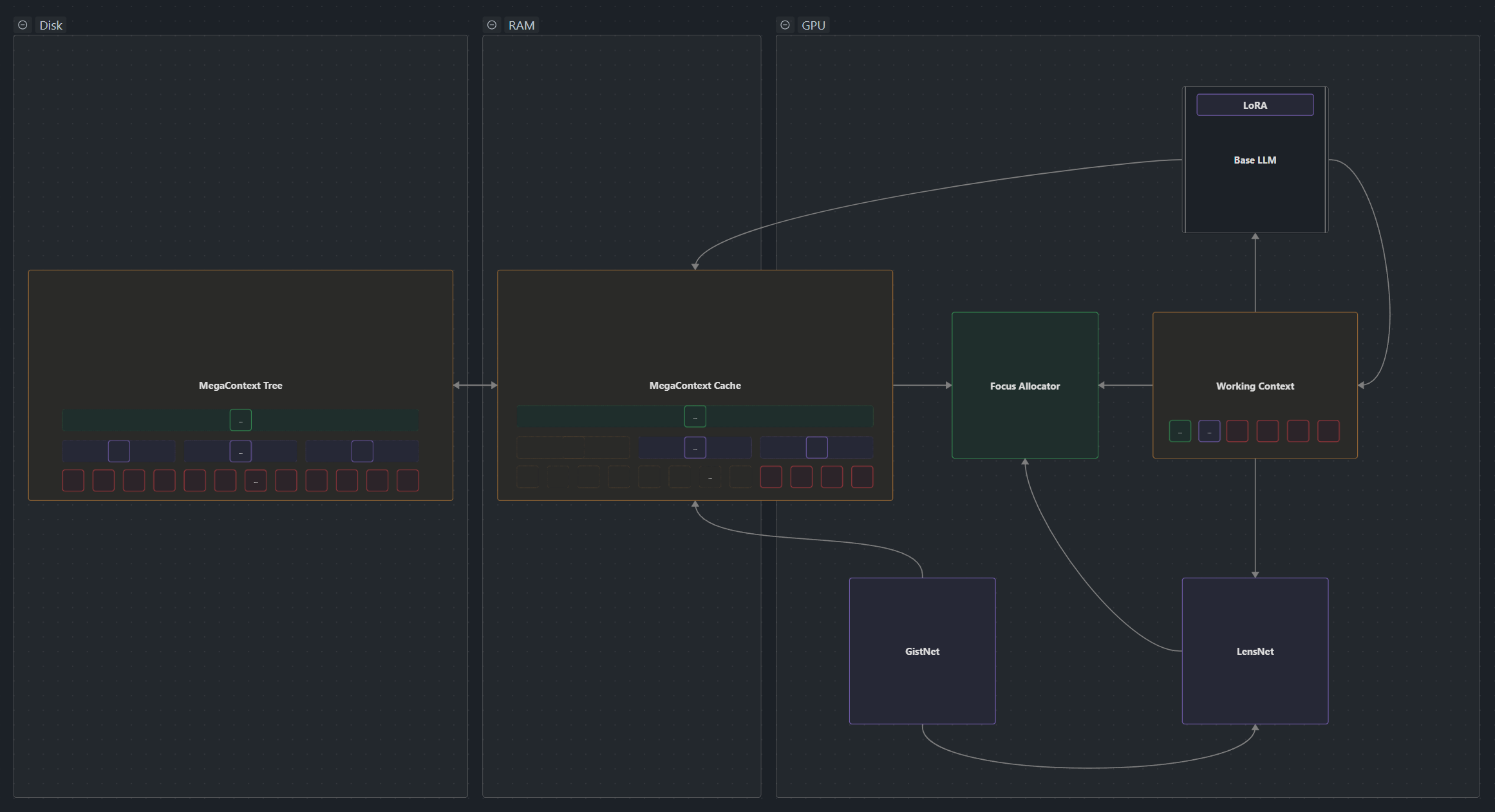 MegaContext virtualizes context by pairing a disk-backed gist tree called the MegaContext Tree with a budgeted working context governed by GistNet, LensNet, and the Focus Allocator. This two-context architecture (1) separates concerns between long-term storage and active processing.
Implementation note: The current notebook prototype lives under
src/megacontext/and implements only the minimal pieces (gistnet, basic runtime wrappers). The full production stack will move into the nanochat fork per the MegaContext PRD Index; reference those PRDs when you need the plan-of-record contracts.
It separates a model’s context into a MegaContext Tree (stored on disk) and a Working Context (on GPU). A learned GistNet model is used to build the MegaContext Tree as a hierarchy of gists [5, 7]. The Working Context compresses the MegaContext Tree into a fixed-size mix of tokens and gists that are used for inference.
To dynamically adapt level of detail, a learned LensNet model [2, 3], continuously/incrementally refocuses the MegaContext Tree onto the Working Context, giving the model effectively infinite memory at constant compute with automatic context management.
- Dual contexts: MegaContext Tree tree vs. Working Context.
- Compression: GistNet builds hierarchical gists aligned with base embeddings.
- Focus/Defocus: LensNet scores working entries; Focus Allocator adjusts detail. Advanced focus layouts (multi-head, staging) are outlined in Multi-headed Focus.
- See also: Runtime Loop for execution, POC Architecture for interfaces.
Table of Contents
- Why Two Contexts?
- The Two-Context Architecture Explained
- Detailed Context Comparison
- How the Contexts Interact
- Data Flow Between Contexts
- Why This Architecture Enables System Properties
- Core Components
- Runtime Lifecycle
- Key Terms & Invariants
- Document Roadmap
Why Two Contexts?
The Fundamental Problem
Large language models face an inherent trade-off between memory capacity and computational efficiency:
1. Fixed Context Windows: Traditional LLMs have a fixed context window (e.g., 4k, 8k, 32k tokens) [12]. Once you exceed this limit, you must either: - Truncate old information (losing history) - Use sliding windows (losing distant context) [12] - Compress everything equally (losing important details)
-
Uniform Attention Cost: Standard transformer attention has O(n²) complexity, where n is the context length. Every token attends to every other token with equal computational cost, regardless of relevance [17].
-
Static Representation: Once text is processed, its representation is fixed. You cannot dynamically adjust the level of detail based on changing relevance as the conversation evolves [9, 11].
The Two-Context Solution
MegaContext solves these problems by separating concerns into two complementary contexts:
MegaContext Tree: The “Hard Drive” of Memory [1]
- Purpose: Store the complete history indefinitely
- Storage: Disk-backed (RAM for POC), hierarchical structure [1]
- Capacity: Effectively unlimited (millions to billions of tokens)
- Access Pattern: Random access, multi-resolution
- Cost Model: Storage cost only, no computation per token
Working Context: The “RAM” of Active Memory
- Purpose: Provide the relevant subset for immediate inference [9]
- Storage: GPU memory, flat sequence [14]
- Capacity: Fixed budget (8k-32k tokens)
- Access Pattern: Sequential processing (left-to-right)
- Cost Model: Full attention cost during inference [17]
Why This Separation Is Necessary
1. Scalability: You cannot fit millions of tokens in GPU memory or process them with O(n²) attention [17] in real-time.
2. Efficiency: Most historical context is not relevant for the current task. Processing everything equally is wasteful [9].
3. Adaptability: Relevance changes over time. Something unimportant earlier may become critical later. The system needs to dynamically refocus.
4. Practicality: Consumer-grade applications at 100M+ context lengths require sub-linear memory and compute scaling.
The Key Insight
The two-context architecture recognizes that there are fundamentally different requirements for:
- Long-term storage (complete, persistent, multi-resolution)
- Active processing (focused, fixed-size, high-detail where needed)
By separating these concerns, MegaContext can optimize each independently while maintaining a coherent view of the entire interaction history.
The Two-Context Architecture Explained
How They Work Together
- GistNet compresses incoming tokens into the MegaContext Tree hierarchy
- LensNet + Focus Allocator selects which parts of the tree to load into Working Context
- Base LLM operates only on the Working Context (remains frozen, unmodified)
- As new tokens are generated, they flow back into the MegaContext Tree
- The cycle repeats, continuously refocusing the Working Context
Detailed Context Comparison
MegaContext Tree vs. Working Context
| Aspect | MegaContext Tree | Working Context |
|---|---|---|
| Purpose | Long-term storage of complete history | Active processing window for inference |
| Storage Location | Disk (RAM in POC) | GPU memory |
| Capacity | Effectively unlimited (millions-billions of tokens) | Fixed budget: 8k-32k tokens |
| Structure | Hierarchical tree (LOD0→LOD1→LOD2→LOD3…) | Flat, contiguous sequence |
| Content | All tokens + all gists at all levels | Mixed: selected tokens and gists |
| Granularity | Multi-resolution (32:1 compression per level) | Variable per entry (LOD0, LOD1, LOD2, etc.) |
| Access Pattern | Random access to any node | Sequential processing (left-to-right) |
| Mutability | Append-only (grows monotonically) | Dynamic (refocused continuously) |
| Temporal Coverage | Complete: every moment since conversation start | Selective: contiguous but variable detail |
| Computational Cost | No inference cost (storage only) | Full attention cost during decode |
| Update Frequency | Block-aligned (every 32 tokens) | Every decode step (via refocus) |
| Persistence | Permanent (survives across sessions) | Ephemeral (rebuilt each step) |
| Visibility to Base LLM | Invisible (never seen directly) | Fully visible (only thing LLM sees) |
| Data Format | Tree nodes with parent/child pointers | Embedding sequence (4096-dim vectors) |
| Indexing | Tree coordinates (level, position) | Linear array (0 to W_max) |
| Compression Method | Hierarchical gisting via GistNet | No compression (but entries may be gists) |
| Detail Control | Implicit (by level) | Explicit (selected by LensNet/FA) |
| Memory Overhead | ~1.5-2x of raw tokens (tree structure) | Exactly W_max embeddings |
| Latency | Disk I/O (negligible for RAM) | Zero (already in GPU) |
| Parallelism | Can build gists in parallel | Sequential attention |
| Failure Mode | Disk full (rare at GB scales) | Budget exceeded (handled by FA) |
| Optimization Target | Minimize ΔNLL (compression loss) | Maximize task performance |
Detailed Breakdown
MegaContext Tree Structure
The MegaContext Tree is a hierarchical compression of the complete history:
Level 3:  ●─────────●─────────●        (each covers 32,768 tokens)
          │         │         │
Level 2:  ●──●──●──●──●──●──●──●      (each covers 1,024 tokens)
          │  │  │  │  │  │  │  │
Level 1:  ●●●●●●●●●●●●●●●●●●●●●●●●    (each covers 32 tokens)
          │││││││││││││││││││││││
Level 0:  [32][32][32][32][32][32]... (raw token blocks)
- LOD0: Raw token blocks (32 tokens each)
- LOD1: Each gist summarizes 32 LOD0 blocks (1,024 tokens → 1 gist)
- LOD2: Each gist summarizes 32 LOD1 gists (32,768 tokens → 1 gist)
- LOD3: Each gist summarizes 32 LOD2 gists (1,048,576 tokens → 1 gist)
Key Properties:
- Each node has at most 32 children
- Compression ratio: 32:1 per level
- Tree depth grows logarithmically: depth = ⌈log₃₂(n)⌉
- Total storage: ~1.5-2× raw tokens (due to redundancy)
Working Context Structure
The Working Context is a contiguous sequence mixing different levels of detail:
Position: [0  ][1  ][2  ][3  ][4  ][5  ][6  ][7  ][8  ]
Content:  [LOD0  ][LOD0  ][LOD1  ][LOD0  ][LOD2  ][LOD1  ][LOD0  ][LOD0  ][LOD0  ]
Cost:     [32  ][32  ][1   ][32  ][1   ][1   ][32  ][32  ][32  ]
Timeline: [0-31][32  ][64  ][96  ][128 ][160 ][192 ][224 ][256 ]
          |----Recent Context----|  |-Mid-| |----Distant Context---|
          (high detail)              (mid)  (low detail)
Key Properties:
- Each entry covers exactly one time interval (no gaps, no overlaps)
- Entries can be at different levels (LOD0, LOD1, LOD2, etc.)
- Total token cost ≤ W_max (enforced by Focus Allocator)
- Temporally contiguous (left-to-right = past-to-present)
- Recent content typically at higher detail (LOD0)
- Distant content typically at lower detail (LOD2, LOD3)
How the Contexts Interact
Three Types of Operations
1. Write: Tokens → MegaContext Tree (via GistNet)
New tokens (from user input or model generation) are written to the MegaContext Tree:
Incoming tokens → LOD0 buffer (32 tokens) → GistNet → LOD1 gist
                                              ↓
                  LOD1 buffer (32 gists) → GistNet → LOD2 gist
                                              ↓
                  LOD2 buffer (32 gists) → GistNet → LOD3 gist
Process:
- Buffer incoming tokens until 32 are collected
- GistNet compresses the 32-token block into a single LOD1 gist
- Store both the LOD0 block and LOD1 gist in the tree
- When 32 LOD1 gists accumulate, compress to LOD2
- Repeat hierarchically up the tree
Triggering:
- Happens automatically as tokens arrive
- Block-aligned (every 32 tokens)
- Independent of Working Context state
2. Read: MegaContext Tree → Working Context (via LensNet + Focus Allocator)
The Working Context is assembled by selecting entries from the MegaContext Tree:
MegaContext Tree (select nodes) → Working Context Assembly → [LOD0][LOD1][LOD0][LOD2]...
                                         ↑
                              LensNet + Focus Allocator
                              (decides what to include)
Process:
- LensNet scores each current Working Context entry for “focus value”
- Positive score = expand to higher detail
- Negative score = collapse to lower detail
- Focus Allocator applies scores while maintaining invariants:
- Contiguity: no temporal gaps
- Budget: total cost ≤ W_max
- Block-alignment: changes respect 32-token boundaries
- Requested entries are fetched from MegaContext Tree
- Working Context is rebuilt with new mix of detail levels
Triggering:
- Every decode step (or every N steps)
- Before each LLM inference pass
- Adaptive based on LensNet scores
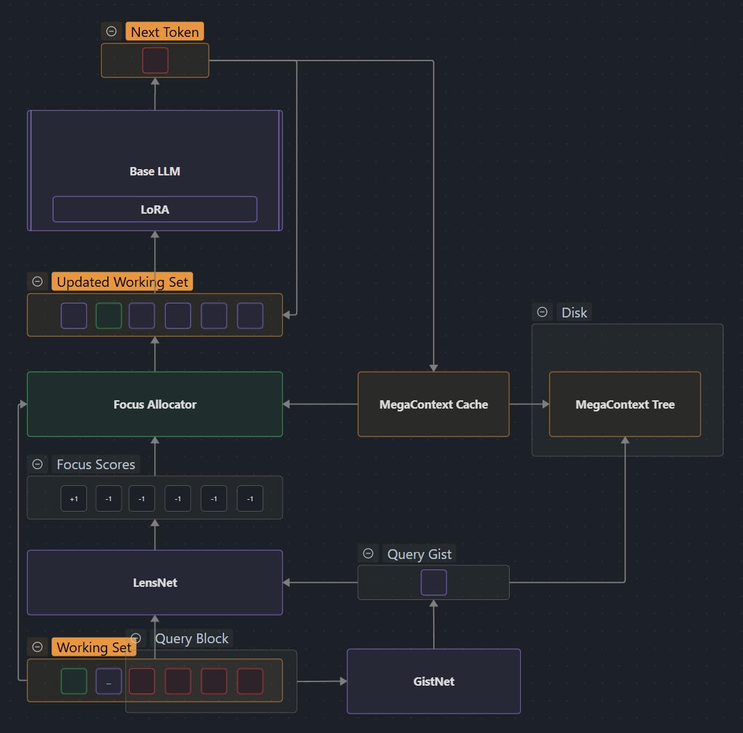
3. Update: Refocusing the Working Context
The Working Context is continuously updated to reflect changing relevance:
Old Working Context → LensNet → Focus Scores → Focus Allocator → New Working Context
         ↑                                                              ↓
         └──────────────────────── (feed to LLM) ────────────────────┘
Example Refocus Cycle:
Step T:   [LOD0][LOD0][LOD1][LOD1][LOD2][LOD0][LOD0]  (current WC)
          ↓
LensNet:  [+1][+2][-1][-2][+3][0 ][0 ]  (focus scores)
          ↓
FA:       expand expand collapse collapse expand keep keep
          ↓
Step T+1: [LOD0][LOD0][LOD0][LOD2][LOD3][LOD0][LOD0]  (updated WC)
                  ^^^ ^^^ ^^^
                 (detail changed)
Why This Matters:
- Relevance changes as conversation evolves
- Something mentioned briefly 10k tokens ago might suddenly become crucial
- System can “zoom in” on newly relevant regions
- Or “zoom out” on distractors to save budget for important content
Data Flow Between Contexts
Complete Data Flow Diagram
┌────────────────────────────────────────────────────────────────────┐
│                         INFERENCE CYCLE                             │
└────────────────────────────────────────────────────────────────────┘

  User Input / Generated Tokens
         │
         ▼
  ┌─────────────┐
  │ Token Buffer│  (accumulate 32 tokens)
  └──────┬──────┘
         │ (every 32 tokens)
         ▼
  ┌─────────────┐
  │   GistNet   │  (compress 32→1)
  └──────┬──────┘
         │
         ▼
  ┌──────────────────────┐
  │  MegaContext Tree    │  (append LOD0 block + LOD1 gist)
  │  ┌───┐ ┌───┐ ┌───┐  │
  │  │LOD3 │─│LOD2 │─│LOD1 │  │
  │  └───┘ └─┬─┘ └─┬─┘  │
  │          │     │     │
  │        ┌─┴─────┴─┐  │
  │        │ LOD0 Blocks│  │
  │        └─────────┘  │
  └──────────┬───────────┘
             │ (read selective entries)
             ▼
  ┌─────────────────────┐
  │  Working Context    │
  │  [LOD0][LOD1][LOD0][LOD2]   │  ◄─────┐
  └──────────┬───────────┘        │
             │                    │
             ▼                    │ (refocus)
  ┌─────────────────────┐        │
  │      LensNet        │        │
  │  (score relevance)  │        │
  └──────────┬───────────┘        │
             │                    │
             ▼                    │
  ┌─────────────────────┐        │
  │  Focus Allocator    │────────┘
  │ (expand/collapse)   │
  └──────────┬───────────┘
             │
             ▼
  ┌─────────────────────┐
  │   Frozen Base LLM   │  (inference)
  │   (e.g., Llama)     │
  └──────────┬───────────┘
             │
             ▼
    Next Token(s) ─────┘ (loop back to buffer)
Step-by-Step Data Flow
Phase 1: Token Ingestion
1. User types: "What did we discuss about machine learning?"
   └─> Buffer: ["What", "did", "we", "discuss", "about", ...]

2. Buffer fills to 32 tokens
   └─> GistNet input: 32 token embeddings [e₁, e₂, ..., e₃₂]

3. GistNet compresses
   └─> LOD1 gist: single embedding [g₁]

4. Write to MegaContext Tree
   ├─> LOD0 node: [e₁, e₂, ..., e₃₂] (32 embeddings)
   └─> LOD1 node: [g₁] (1 embedding, parent of LOD0)

5. Update tree metadata
   ├─> ΔNLL: compression loss metric
   ├─> Timestamps: token positions
   └─> Parent/child pointers
Phase 2: Working Context Assembly
1. LensNet reads current Working Context
   └─> Input: [WC₁, WC₂, ..., WCₙ] + [tail gists from MC Tree]

2. LensNet computes focus scores
   └─> Output: [score₁, score₂, ..., scoreₙ]
        └─> score > 0: expand (more detail)
        └─> score < 0: collapse (less detail)

3. Focus Allocator processes scores
   ├─> For each positive score:
   │   ├─> Fetch children from MegaContext Tree
   │   ├─> Replace LOD1 gist with 32 LOD0 blocks
   │   └─> Check budget: cost ≤ W_max?
   │
   └─> For each negative score:
       ├─> Find parent in MegaContext Tree
       ├─> Replace 32 LOD0 blocks with 1 LOD1 gist
       └─> Frees budget for other expansions

4. New Working Context assembled
   └─> [mix of LOD0, LOD1, LOD2, LOD3 entries]
        ├─> Contiguous in time (no gaps)
        └─> Within budget (total cost ≤ W_max)
Phase 3: Inference
1. Working Context fed to base LLM
   └─> Input: sequence of embeddings
        ├─> LOD0 entries: raw token embeddings
        └─> LOD1/LOD2/LOD3 entries: gist embeddings
        (LLM cannot distinguish - same embedding dimension)

2. LLM runs attention
   └─> Full O(n²) attention over Working Context only
        └─> n = (W_max / avg_entry_cost) ≈ 256-1024 entries

3. LLM generates next token
   └─> Output: new token embedding [e_new]

4. Token loops back to Phase 1
   └─> Added to buffer, eventually compressed to tree
Data Flow Properties
1. Unidirectional Write Path:
- Tokens → MegaContext Tree (via GistNet)
- Tree is append-only, never modified
2. Bidirectional Read Path:
- MegaContext Tree → Working Context (fetch entries)
- Working Context → LensNet (compute scores)
- Scores → Focus Allocator → Updated Working Context
3. Isolation:
- Base LLM never sees MegaContext Tree directly
- Base LLM only operates on Working Context
- GistNet never sees Working Context
- LensNet never modifies MegaContext Tree
4. Cycle Time:
- GistNet: O(32) tokens to trigger
- LensNet: O(1) decode step (or every N steps)
- Base LLM: O(1) token generation
Why This Architecture Enables System Properties
1. Unbounded Context Length ✓
How: MegaContext Tree stores complete history on disk with logarithmic depth.
Math:
- Tree depth = ⌈log₃₂(n)⌉
- For 1M tokens: depth = 4 levels
- For 1B tokens: depth = 6 levels
- Storage: ~1.5n embeddings (linear)
Why Two Contexts Are Essential:
- Cannot store 1B tokens in GPU (would require ~4TB)
- Cannot process 1B tokens with O(n²) attention (would take hours per token)
- Disk storage is cheap and scales linearly
- Working Context stays fixed size regardless of total history
2. Constant Compute Cost ✓
How: Working Context has fixed budget W_max; base LLM complexity is O(W_max²).
Math:
- Attention cost: O(W_max²) = O(1) for fixed W_max
- Example: W_max = 32k tokens → ~1B FLOPs per decode
- Independent of total history length (could be 1M or 1B tokens)
Why Two Contexts Are Essential:
- Base LLM only sees Working Context (W_max tokens)
- MegaContext Tree is outside the inference path
- No matter how much history accumulates, inference cost stays constant
3. Dynamic Focus/Defocus ✓
How: LensNet scores relevance; Focus Allocator swaps detail levels.
Example:
T=0:  "My cat's name is Fluffy. [9500 tokens about other topics]"
      Working Context: [LOD3 gist] (low detail)

T=9500: "What was my cat's name?"
      LensNet detects query, scores LOD3 gist highly
      Focus Allocator: LOD3 → LOD2 → LOD1 → LOD0
      Working Context: [LOD0 tokens: "My cat's name is Fluffy"]
Why Two Contexts Are Essential:
- MegaContext Tree preserves all detail at all levels (lossless traversal)
- Working Context can swap between levels without re-encoding
- One-way compression (e.g., RAG summaries) cannot “zoom back in”
- Static context windows cannot adjust detail post-hoc
4. Lossy-Yet-Restorable Compression ✓
How: Gists compress 32→1 (lossy) but original tokens remain in tree (restorable).
Compression Cascade:
32 tokens → 1 LOD1 gist (97% compression, small ΔNLL)
32 LOD1 gists → 1 LOD2 gist (97% compression, medium ΔNLL)
32 LOD2 gists → 1 LOD3 gist (97% compression, higher ΔNLL)
Restoration:
Need more detail? Traverse tree:
LOD3 gist → fetch 32 LOD2 children → fetch 32×32 LOD1 children → fetch 32×32×32 LOD0 tokens
Why Two Contexts Are Essential:
- MegaContext Tree stores both compressed (gists) and original (tokens)
- Working Context can dynamically choose which representation to use
- Trade-off: budget (use gist) vs. fidelity (use tokens)
- Not possible with single context (must choose one representation)
5. Sub-Linear Memory Scaling ✓
How: MegaContext Tree in cheap disk/RAM; Working Context in expensive GPU RAM.
Memory Breakdown:
MegaContext Tree:  ~1.5n embeddings × 16KB each = 24n bytes (disk/RAM)
Working Context:   W_max embeddings × 16KB each = constant (GPU)
LensNet + GistNet: Small models (~10-100M params = 40-400MB GPU)

Example (1B tokens):
- MC Tree: 1.5B × 16KB = 24GB (RAM) ✓ affordable
- WC: 32k × 16KB = 512MB (GPU) ✓ affordable
- Total GPU: ~1GB (leaves 23GB for base LLM)
Why Two Contexts Are Essential:
- GPU memory is 10-100× more expensive than RAM
- Cannot afford to keep all history in GPU
- Disk/RAM storage scales to TBs for pennies
- Working Context uses GPU efficiently (only what’s needed)
6. No Retraining of Base Model ✓
How: Base LLM remains frozen; operates on same embedding space.
Architecture:
Base LLM (frozen)
     ↑
     │ (same embeddings)
     │
Working Context ← mix of tokens + gists
                      ↑
                    GistNet (learned)
                      ↑
                  Raw Tokens
Why Two Contexts Are Essential:
- GistNet learns to produce embeddings that “look like” base model tokens
- Base LLM cannot tell the difference between LOD0 tokens and LOD1/LOD2/LOD3 gists
- Working Context is the “adapter layer” - provides abstraction
- MegaContext Tree is GistNet’s domain - invisible to base model
- Separation allows independent optimization of each component
7. Multi-Resolution Access ✓
How: Tree structure provides access at any granularity (LOD0, LOD1, LOD2, LOD3).
Access Patterns:
Coarse scan:  Read LOD3 gists (1 per 1M tokens) → fast overview
Medium scan:  Read LOD2 gists (1 per 32k tokens) → section-level
Fine scan:    Read LOD1 gists (1 per 1k tokens) → paragraph-level
Full detail:  Read LOD0 tokens (all 32 tokens) → word-level
Example Use Case:
Query: "Find all discussions about Python optimization"

1. Scan all LOD3 gists (1000 in 1B-token history) → 1000 gists
2. Identify 10 relevant LOD3 regions
3. Scan their LOD2 children (10 × 32 = 320 gists)
4. Identify 5 most relevant LOD2 regions
5. Expand to LOD0 for detailed reading (5 × 1024 tokens = 5120 tokens)

Total cost: 1000 + 320 + 5120 = 6440 tokens (vs. 1B tokens for full scan)
Why Two Contexts Are Essential:
- MegaContext Tree provides multi-resolution storage
- Working Context provides multi-resolution representation
- Can query coarsely, then zoom in selectively
- Not possible with flat context or RAG (fixed retrieval granularity)
Core Components
1. MegaContext Tree
Purpose: Persistent, hierarchical storage of complete conversation history.
Key Responsibilities:
- Store all tokens (LOD0) and all gists (LOD1, LOD2, LOD3, …)
- Maintain parent-child relationships
- Support random access at any level
- Track metadata (ΔNLL, timestamps, etc.)
- Persist across sessions
See: MegaContext Tree, Storage Format, Tree Operations
2. Working Context
Purpose: Active, budget-constrained window for LLM inference.
Key Responsibilities:
- Maintain contiguous temporal coverage
- Mix tokens and gists optimally
- Stay within token budget (W_max)
- Provide embedding sequence to base LLM
- Update continuously via refocusing
See: Working Context, Working Context Assembly, Working Context Refocusing
3. GistNet
Purpose: Learned compression model that builds the tree hierarchy.
Key Responsibilities:
- Compress 32 tokens → 1 gist (LOD0 → LOD1)
- Compress 32 gists → 1 gist (LOD1 → LOD2, LOD2 → LOD3, …)
- Minimize ΔNLL (compression loss)
- Align gists with base model embedding space
- Train via self-supervised learning
Architecture:
- Input: 32 embeddings (4096-dim each)
- Output: 1 embedding (4096-dim)
- Model: Transformer encoder (6-12 layers, 512-2048 hidden dim) [2]
- Training: Minimize perplexity of next-token prediction [21]
See: GistNet, GistNet Architecture Details, GistNet Training
4. LensNet
Purpose: Learned scoring model that determines what to focus on.
Key Responsibilities:
- Score each Working Context entry for relevance
- Predict which entries should be expanded/collapsed
- Adapt to task dynamics (queries, continuations, etc.)
- Balance exploration vs. exploitation
- Train via reinforcement learning or task supervision
Architecture:
- Input: Working Context + tail gists (context representation)
- Output: Focus scores (one per entry)
- Model: Transformer encoder (4-8 layers, 256-1024 hidden dim)
- Training: Maximize task reward (e.g., downstream NLL)
See: LensNet, LensNet Scoring, LensNet Training
5. Focus Allocator
Purpose: Deterministic algorithm that applies LensNet scores to refocus Working Context.
Key Responsibilities:
- Enforce contiguity (no temporal gaps)
- Enforce budget (total cost ≤ W_max)
- Expand high-scoring entries (fetch children)
- Collapse low-scoring entries (replace with parent)
- Handle edge cases (boundary conditions, buffer limits)
Algorithm:
def focus_allocator(working_context, scores, budget):
    # Sort scores descending
    expansions = [(i, score) for i, score in enumerate(scores) if score > 0]
    expansions.sort(key=lambda x: x[1], reverse=True)

    # Greedily expand until budget exhausted
    for i, score in expansions:
        if can_expand(working_context[i], budget):
            working_context[i] = expand(working_context[i])
            budget -= expansion_cost(working_context[i])

    # Collapse low-scoring entries to free budget
    collapses = [(i, score) for i, score in enumerate(scores) if score < 0]
    for i, score in collapses:
        if should_collapse(working_context[i]):
            working_context[i] = collapse(working_context[i])
            budget += collapse_savings(working_context[i])

return working_contextSee: Focus Allocator, Focus Allocator Strategies
6. Base LLM
Purpose: Frozen language model that performs inference.
Key Characteristics:
- Unchanged: No modifications to architecture or weights
- Embeddings: Operates on same embedding space as training
- Input: Working Context (mix of tokens and gists)
- Output: Next token probabilities
- Oblivious: Cannot distinguish tokens from gists
Examples: Llama, GPT, Claude (frozen, no finetuning)
Runtime Lifecycle
System Initialization
1. Load base LLM (frozen weights)
2. Load GistNet (pre-trained weights)
3. Load LensNet (pre-trained weights)
4. Initialize MegaContext Tree (empty or from checkpoint)
5. Initialize Working Context (empty)
6. Ready for first token
Token Processing Loop
LOOP (for each new token):

    1. TOKEN ARRIVAL
       ├─> User input or model generation
       └─> Add to buffer

    2. TREE UPDATE (every 32 tokens)
       ├─> GistNet: compress 32 tokens → 1 LOD1 gist
       ├─> Write LOD0 block + LOD1 gist to tree
       └─> Recursively compress LOD1→LOD2, LOD2→LOD3, etc.

    3. REFOCUS (every decode step or every N steps)
       ├─> LensNet: score Working Context entries
       ├─> Focus Allocator: apply scores
       │   ├─> Expand high-score entries (fetch children)
       │   └─> Collapse low-score entries (replace with parent)
       └─> Rebuild Working Context with new entries

    4. INFERENCE
       ├─> Feed Working Context to base LLM
       ├─> LLM generates next token
       └─> Loop back to step 1

END LOOP
Example Execution Trace
T=0: User: "Tell me about Paris"
     └─> Buffer: ["Tell", "me", "about", "Paris"]
     └─> Working Context: [LOD0: "Tell", "me", "about", "Paris"]
     └─> LLM: "Paris is the capital..."

T=32: Buffer full → GistNet compresses
     └─> MC Tree: [LOD0: 32 tokens], [LOD1: gist_1]
     └─> Working Context: [LOD0: recent 32 tokens]

T=1000: User: "What about London?"
     └─> LensNet scores Paris discussion (low relevance)
     └─> Focus Allocator: collapse LOD0 → LOD1
     └─> Working Context: [LOD1: gist_Paris], [LOD0: recent tokens]
     └─> More budget available for new London discussion

T=1050: User: "Compare Paris and London"
     └─> LensNet scores Paris gist (high relevance)
     └─> Focus Allocator: expand LOD1 → LOD0
     └─> Working Context: [LOD0: Paris details], [LOD0: London details]
     └─> LLM can compare with full context
Key Terms & Invariants
Key Terms
- LOD0: Raw token blocks (32 tokens each)
- LOD1/LOD2/LOD3: Gist levels (each compresses 32 children)
- Gist: Single embedding that summarizes 32 child embeddings
- Entry: One item in Working Context (can be LOD0, LOD1, LOD2, or LOD3)
- Cost: Number of base tokens represented (LOD0=32, LOD1=1, LOD2=1, LOD3=1)
- Budget (W_max): Maximum token cost for Working Context
- ΔNLL: Compression loss (increase in perplexity due to gisting)
- Focus: Expand entry to higher detail (replace gist with children)
- Defocus: Collapse entry to lower detail (replace children with gist)
- Contiguity: Working Context covers time without gaps
- Refocus: Update Working Context by applying focus/defocus operations
Core Invariants
MegaContext Tree Invariants:
- Append-only: Nodes are never deleted or modified
- Complete: All LOD0 blocks are stored (no truncation)
- Hierarchical: Each non-leaf node has ≤32 children
- Aligned: LOD0 blocks start at multiples of 32
- Redundant: Both compressed (gists) and original (tokens) are stored
Working Context Invariants:
- Contiguous: Covers [start_pos, end_pos] without gaps
- Budgeted: ∑(entry_cost) ≤ W_max
- Mixed: Entries can be at any level (LOD0, LOD1, LOD2, LOD3)
- Temporal: Left-to-right = past-to-present
- Aligned: Each entry covers exactly one tree node’s time span
System Invariants:
- Isolation: Base LLM never accesses MegaContext Tree directly
- Constant Compute: Inference cost = O(W_max²), independent of history
- Lossless Paths: Can always traverse tree to restore original tokens
- Embedding Consistency: Gists are in same embedding space as tokens
- No Retraining: Base LLM weights are frozen, never updated
See: Invariants for complete details
Document Roadmap
This document is the canonical reference for understanding MegaContext’s two-context architecture. For deeper dives into specific aspects:
Architecture Deep Dives
- MegaContext Tree - Complete tree structure and storage
- Working Context - Budget management and assembly
- POC Implementation - Current implementation details
- System Properties - Formal property proofs
Component Details
- GistNet - Compression model design
- GistNet Architecture Details - Network structure
- GistNet Training - Training procedures
- LensNet - Focus scoring model
- LensNet Scoring - Scoring mechanisms
- LensNet Training - Training procedures
- Focus Allocator - Refocusing algorithm
- Focus Allocator Strategies - Allocation policies
Operations
- Tree Operations - Build, query, traverse
- Working Context Assembly - Initial assembly
- Working Context Refocusing - Dynamic updates
- Node Metadata - Metadata tracking
Training & Optimization
- MegaContext End-to-End Training - Joint training strategy
- Telemetry - Metrics and monitoring
Comparisons & Context
- How MegaContext Works - Introductory overview
- MegaTexture Analogy - Visual intuition
- Comparisons - vs. RAG, sparse attention, etc.
- Related Work - Academic context
Summary
The two-context architecture is the foundation of MegaContext’s ability to provide unbounded memory at constant compute:
- MegaContext Tree stores the complete history hierarchically on disk
- Working Context provides a fixed-size, dynamically-refocused view for inference
- GistNet builds the tree by compressing tokens into gists
- LensNet + Focus Allocator adapts the Working Context to changing relevance
- Base LLM operates unchanged on the Working Context
This separation enables:
- ✓ Unbounded context length (millions to billions of tokens)
- ✓ Constant compute cost (O(W_max²) regardless of history)
- ✓ Dynamic focus/defocus (zoom in on relevant regions)
- ✓ Lossy-yet-restorable compression (gists + original tokens)
- ✓ Sub-linear memory scaling (disk for tree, GPU for working set)
- ✓ No retraining of base model (frozen weights)
- ✓ Multi-resolution access (coarse scan → fine detail)
The key insight: By separating long-term storage from active processing, MegaContext can optimize each independently while maintaining a coherent view of the entire interaction history. This is not possible with a single-context architecture.
References
- MegaTexture (Carmack, 2007) — Analysis — Virtual texturing system that inspired the core hierarchical streaming architecture
- Perceiver (Jaegle et al., 2021) — Analysis — Latent cross-attention bottleneck architecture
- Perceiver IO (Jaegle et al., 2021) — Analysis — Query-based decoding for arbitrary structured outputs
- Gist Tokens (Mu et al., 2023) — Analysis — Learned prompt compression via attention masking
- Compressive Transformer (Rae et al., 2019) — Analysis — Long-term compressed memory for transformers
- RAG (Lewis et al., 2020) — Analysis — Retrieval-augmented generation baseline
- Memorizing Transformers (Wu et al., 2022) — Analysis — kNN-augmented approximate retrieval
- Transformer-XL (Dai et al., 2019) — Analysis — Segment-level recurrence and relative positional encoding
- RoPE (Su et al., 2021) — Analysis — Rotary position embeddings used throughout MegaContext
- Flash Attention (Dao et al., 2022) — Analysis — IO-aware exact attention algorithm
- Knowledge Distillation (Hinton et al., 2015) — Analysis — Teacher-student framework for GistNet training
See Related Work for the complete bibliography of all research papers referenced throughout the documentation.
This document is the definitive guide to MegaContext’s two-context architecture. All other documentation should reference this page for architectural fundamentals.